IMAGES FROM THE ENTIRE BOOK
please check gray text for attribution and licensing restrictions
images in copyright are not available for download

	FIGURE 0.1
	Partition and unification of territorial states since 1945
	William Rankin Creative Commons BY-NC-SA
	FIGURE 0.2
	Typical ocean claims under the UN Convention on the Law of the Sea
	William Rankin Creative Commons BY-NC-SA
	FIGURE 0.3
	Territorial claims in the Arctic Ocean, 1971 and 2015
	William Rankin Creative Commons BY-NC-SA
	FIGURE 0.4
	Telecommunications cables in 2009 (detail)
	Telegeography Creative Commons BY-NC-ND
	FIGURE 1.1
	International Map of the World, Hudson River, 1927
	US Geological Survey Public Domain: US government
	FIGURE 1.2
	International Map of the World adherents as of 1913
	William Rankin Creative Commons BY-NC-SA
	FIGURE 1.3
	A map at 1:2,000,000 – “Northern Great Lakes States" from The National Atlas of the United States of America (1970)
	A map at 1:1,000,000 – International Map of the World, Lake Superior (1966)
	A map at 1:250,000 – Escanaba sheet from series V501 (1967)
	all US Geological Survey Public Domain: US government
	FIGURE 1.4
	Grid of the International Map of the World download grid as a GIS layer
	William Rankin Creative Commons BY-NC-SA
	FIGURE 1.5
	Mapping projects at 1:1,000,000 as of 1905
	from Albrecht Penck, “Fortschritte in der Herstellung einer Erdkarte in Maßtabe 1 : 1 000 000,” Zeitschrift der Gesellschaft für Erdkunde zu Berlin (1905); shading added Public Domain: copyright expired
	FIGURE 1.6
	Symbols for the International Map of the World, as approved in 1909
	from Resolutions and Proceedings of the International Map Committee assembled in London, November, 1909 (London: HMSO, 1910) Public Domain: copyright expired
	FIGURE 1.7
	Symbols for the International Map of the World, as approved in 1913
	from Carte du Monde au Millionième: Comptes Rendus des séances de la deuxième conférence internationale, Paris, décembre 1913 (Paris: Service Géographique, 1914) Public Domain: copyright expired
	FIGURE 1.8
	Comparison of 1909 and 1913 elevation colors for the International Map of the World
	from Resolutions and Proceedings of the International Map Committee assembled in London, November, 1909 (London: HMSO, 1910) and Carte du Monde au Millionième: Comptes Rendus des séances de la deuxième conférence internationale, Paris, décembre 1913 (Paris: Service Géographique, 1914) Public Domain: copyright expired
	FIGURE 1.9
	Responsibility for the International Map of the World in Africa, as approved in 1913
	William Rankin Creative Commons BY-NC-SA
	FIGURE 1.10
	Comparison of symbols for the International Map of the World with other topographic maps of the same era
	William Rankin Creative Commons BY-NC-SA
	FIGURE 1.11
	Typical land-cover symbols from the early twentieth century
	from John Clayton Tracy, Plane Surveying: A Text-book and Pocket Manual (New York: John Wiley & Sons, 1906), 521 Public Domain: copyright expired
	FIGURE 1.12
	Frontispiece to the International Map of the World annual reports
	from Carte du Monde au Millionième: Rapport pour 1921 (Southampton: Ordnance Survey, 1922) Public Domain: copyright expired
	NOTE 1.71
	Members of the International Commission for Air Navigation as of 1939
	William Rankin Creative Commons BY-NC-SA
	FIGURE 1.13
	French aeronautical chart, Chalons (1911)
	from P. Pollacchi, “La carte aéronautique du service géographique de l’armée,” Annales de Géographie 20, no. 112 (1911), plate 18 Public Domain: copyright expired
	FIGURE 1.14
	Aeronautical adaptation of the International Map of the World sheet for London (1934)
	British War Office Public Domain: expired Crown Copyright
	FIGURE 1.15
	Official International Map of the World sheets published before 1939
	William Rankin Creative Commons BY-NC-SA
	FIGURE 1.16
	Unofficial or “provisional” International Map of the World sheets published before 1939
	William Rankin Creative Commons BY-NC-SA
	FIGURE 1.17
	Sources assembled at the American Geographical Society for the Map of Hispanic America.
	American Geographical Society Copyright 1946, renewed 1973
	FIGURE 1.18
	Relative reliability diagram for The Map of Hispanic America — Istmo de Tehuantepec, 1938
	American Geographical Society Public Domain: copyright not renewed
	FIGURE 1.19
	Assembling a portion of the American Geographical Soviety's Map of Hispanic America
	Alfred Eisenstaedt Copyright 1941
	FIGURE 1.20
	Assembling the Map of Hispanic America in the courtyard of the American Geographical Society
	American Geographical Society Copyright 1946, renewed 1973
	FIGURE 2.1
	Number of sheets of the International Map of the World published or revised, 1921–1986 download data in a spreadsheet
	William Rankin Creative Commons BY-NC-SA
	FIGURE 2.2
	Coverage of the International Map of the World as of 1986
	from “Status of Publication of IMW Sheets as at 31 December 1986,” UN Document ST/ESA/SER.D/17, Supplement #3 (Feb 1987) Public Domain: UN publication
	FIGURE 2.3
	The Mercator projection, from a 1938 atlas
	from Rand McNally Ready-Reference Atlas of the World (Chicago, 1938) Public Domain: copyright not renewed
	FIGURE 2.4
	Map illustrating the new strategic importance of polar routes through Alaska during World War II
	Life Magazine Copyright 1942, renewed 1969
	FIGURE 2.5
	Map with bold arrows and a perspective view shows the battle over oil in the Middle East
	Life Magazine Copyright 1941, renewed 1969
	FIGURE 2.6
	Richard Edes Harrison's famous polar map showing the centrality of the United States to the global conflict
	originally in Fortune, March 1942; this link points to the 1944 version in Look At The World Copyright 1942, renewed 1969
	FIGURE 2.7
	Frontispiece to Wendell Willkie's One World, showing his route around the globe
	Simon & Schuster Copyright 1943, renewed 1970
	FIGURE 2.8
	Richard Edes Harrison's views of a spherical earth, ignoring north-up conventions: the view from the US towards Asia, and the view from Europe towards Asia
	from Richard Edes Harrison, Look At The World Copyright 1944, renewed 1971
	FIGURE 2.9
	The United Nations emblem (azimuthal equidistant projection): original lapel pin and present-day version
	US Office of Strategic Services; United Nations Public Domain: US Government / UN
	FIGURE 2.10
	A new oblique Mercator projection showing global air routes without any regional frame
	Geographical Journal Copyright 1941
	FIGURE 2.11
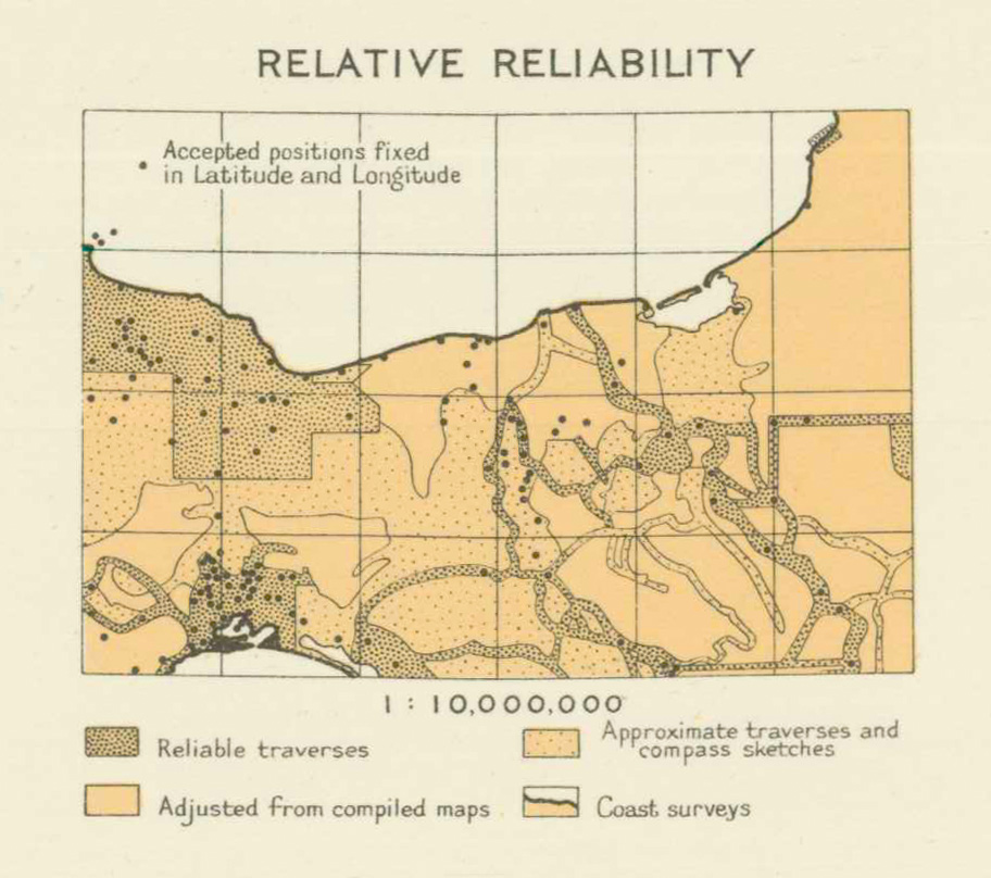
	International Map of the World sheet Istmo de Tehuantepec (1938)
	American Geographical Society Public Domain: copyright not renewed
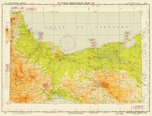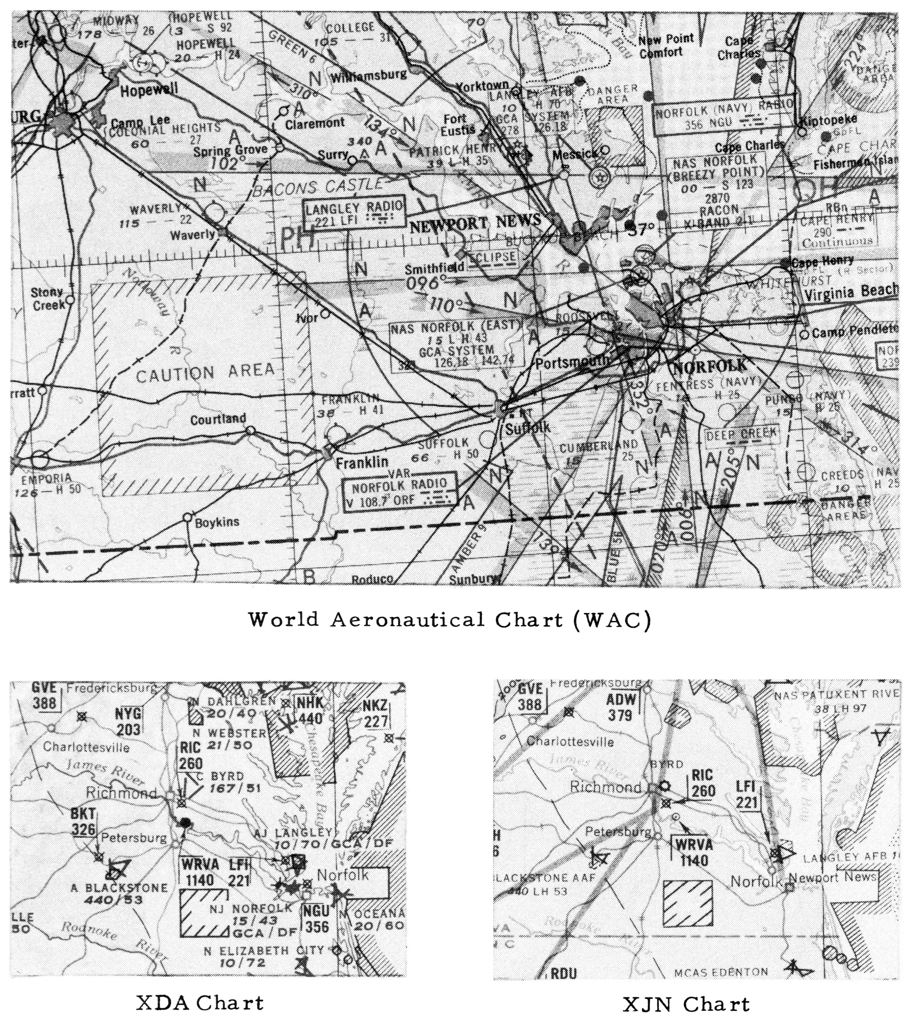
	World Aeronautical Chart sheet Tehuantepec Isthmus (1946)
	US Aeronautical Chart Service Public Domain: US government
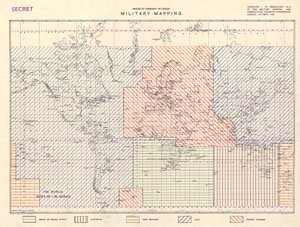
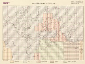
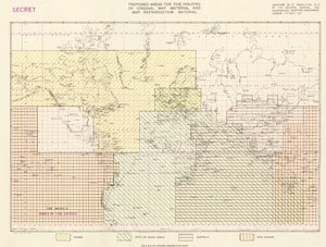
	FIGURE 2.12
	The division of Allied mapping responsibility in 1947: military-topographic maps, aeronautical charts, and storage of reproduction material
	Directorate of Military Survey Copyright 1947
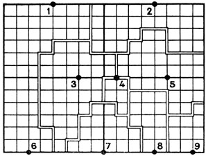
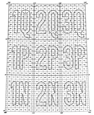
	FIGURE 2.13
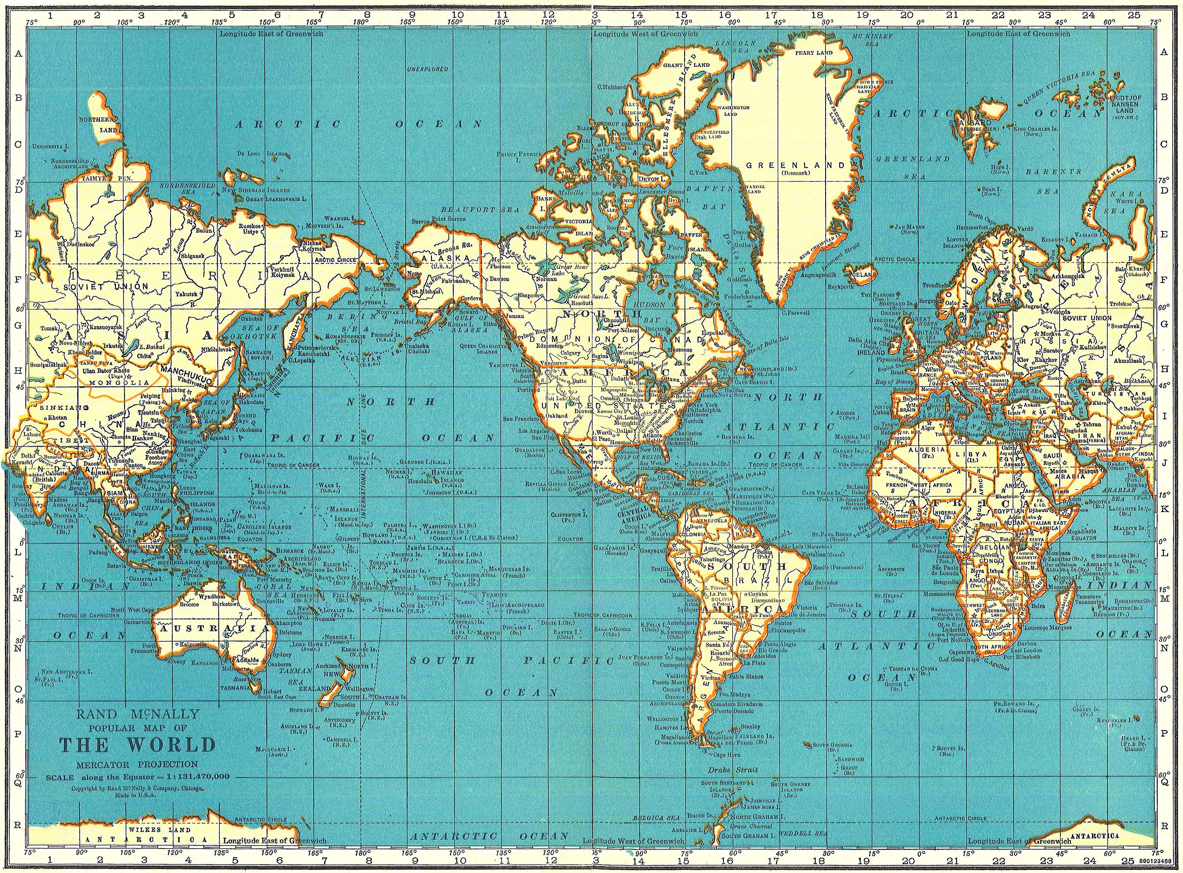
	Comparison of sheet grids for the International Map of the World and the World Aeronautical Chart
	William Rankin Creative Commons BY-NC-SA
	FIGURE 2.14
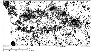
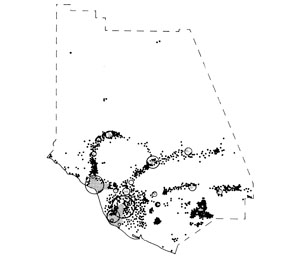
	World Population Maps of Tuscany (top) and Ventura County, California (bottom)
	Geografiska Annaler Copyright 1963
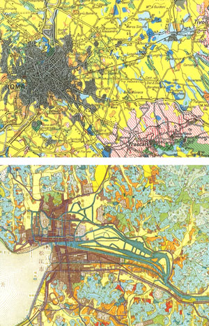
	FIGURE 2.15
	Comparison of World Land-Use Survey maps from central Italy (top) and western Japan (bottom)
	Internationales Jahrbuch für Kartographie Copyright 1968
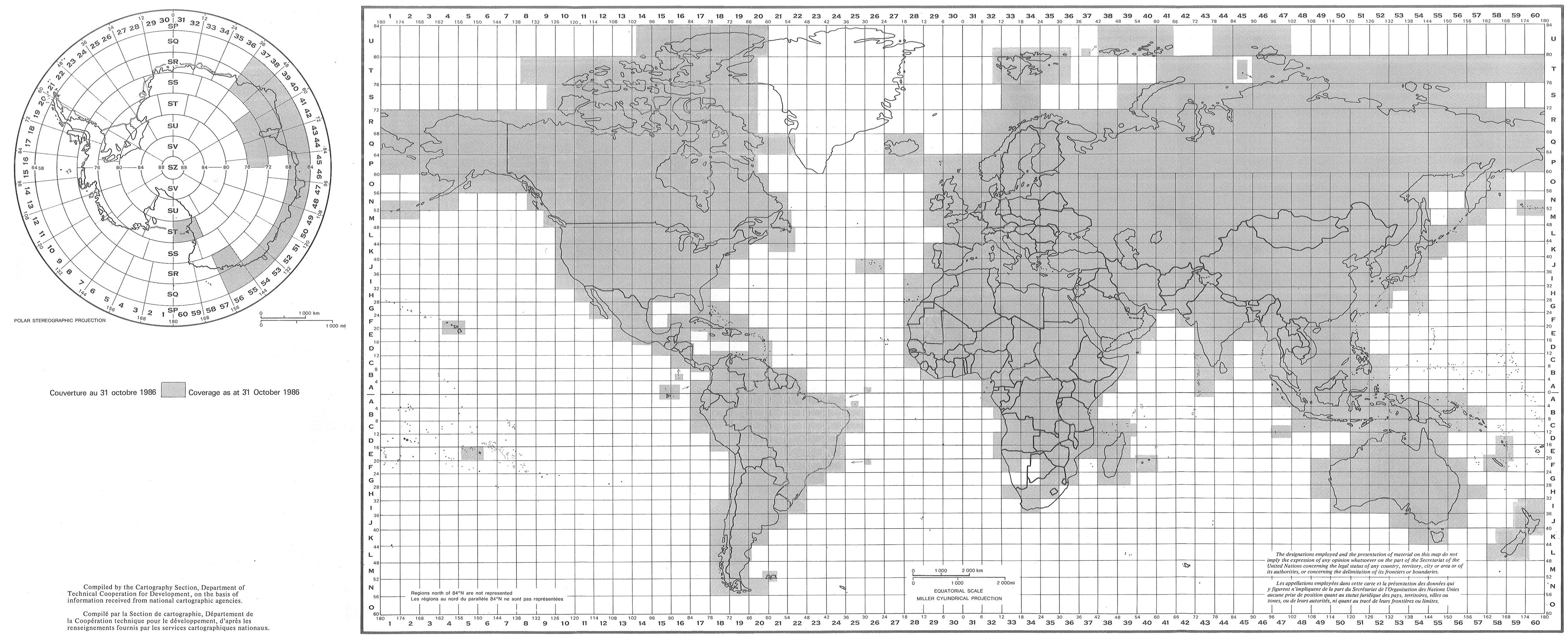
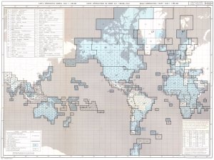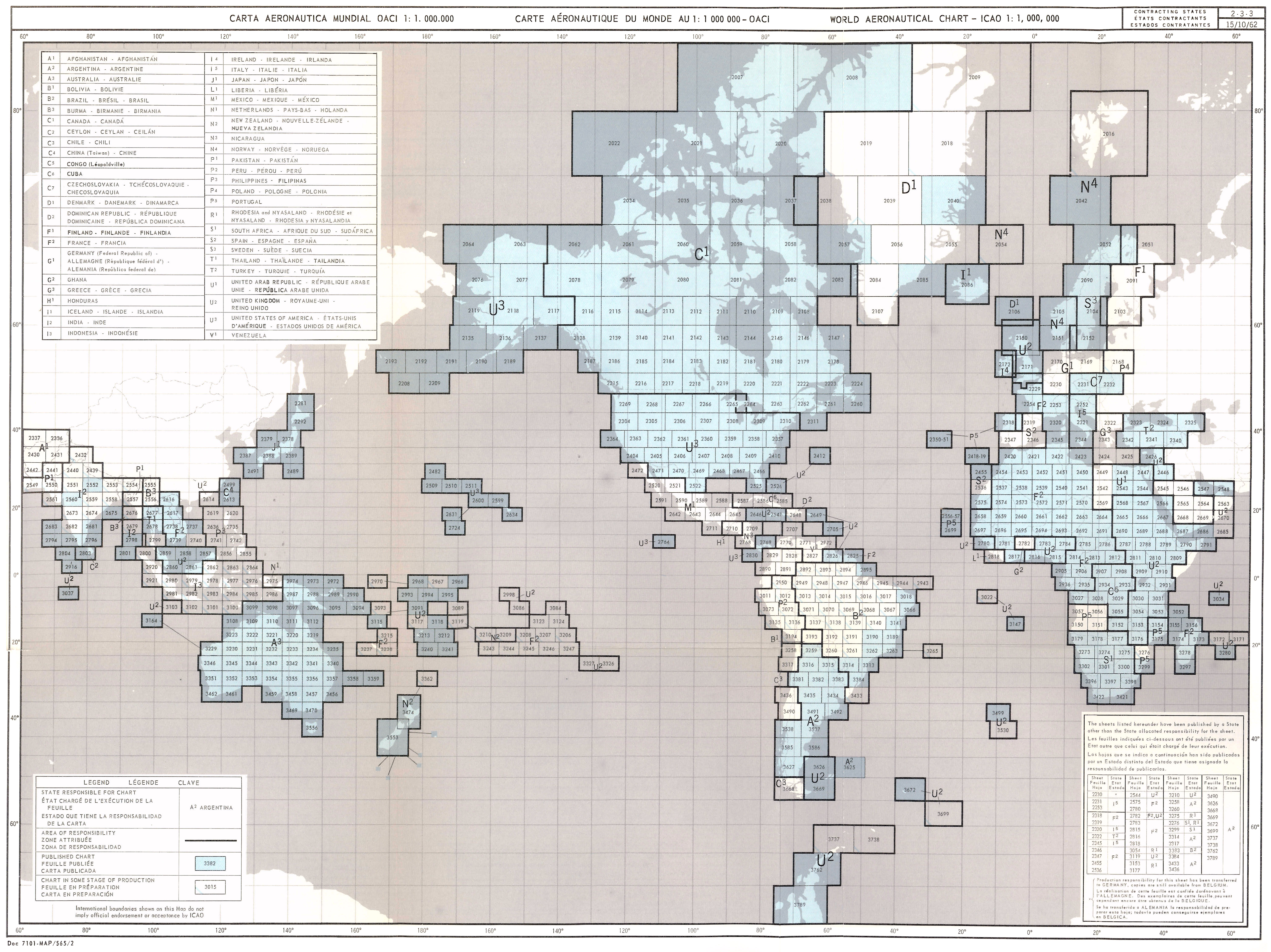
	FIGURE 2.16
	Sheet index for the International World Aeronautical Chart: March and October 1962
	International Civil Aviation Organization Public Domain: UN publication
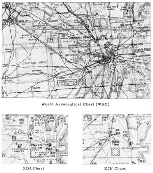	FIGURE 2.17
	Design alternatives for the World Aeronautical Chart tested for the US Office of Naval Research in 1952
	from John E. Murray and Rolland H. Waters, “The Design of Aeronautical Charts II,” Navigation (US) 3 (Dec 1952), 193 Public Domain: copyright not renewed
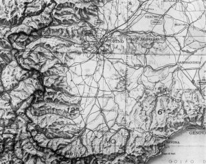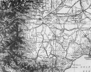
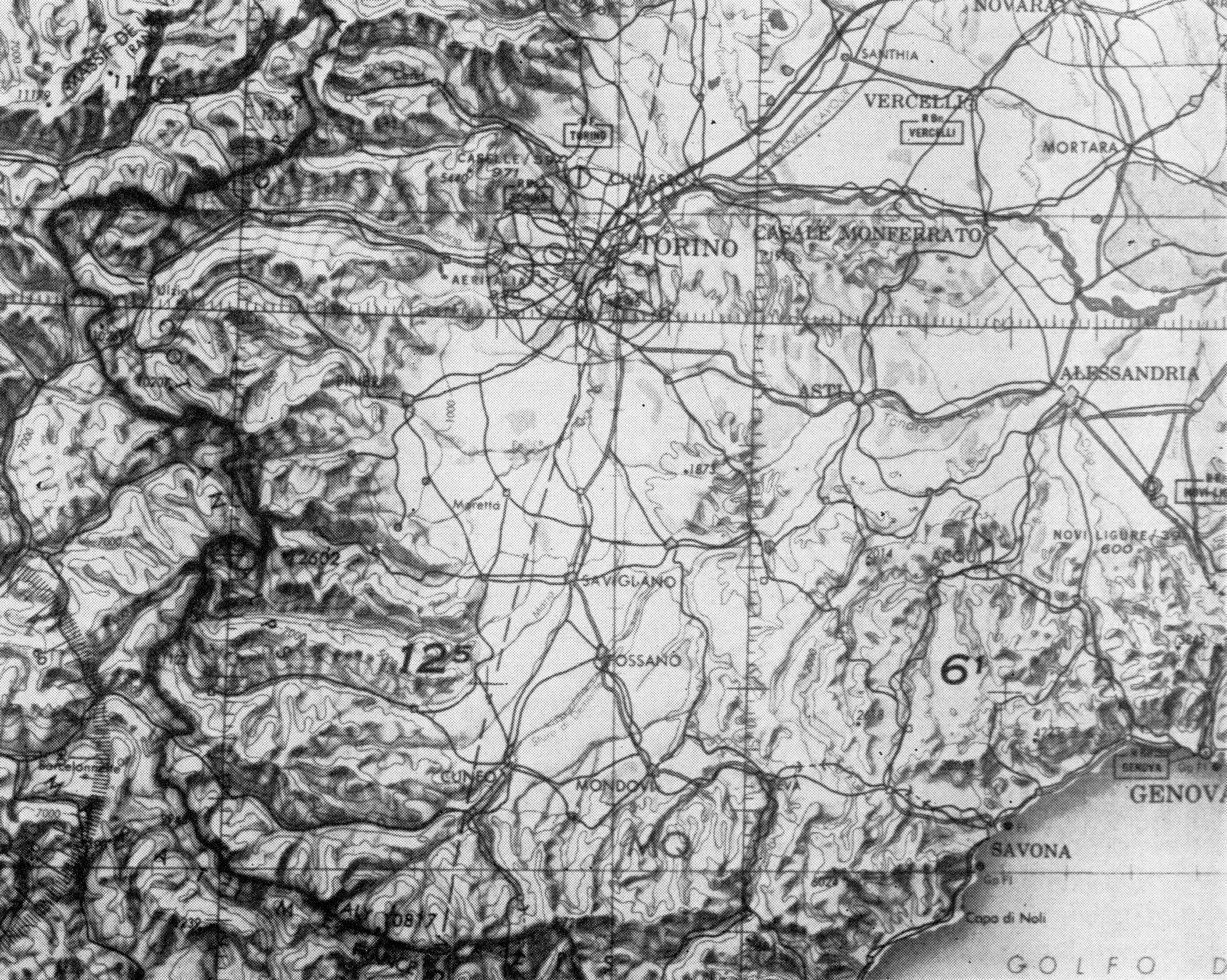
	FIGURE 2.18
	Comparison of the design of American World Aeronautical Charts in 1948 and 1957 (both maps show the same area in northern Italy)
	from Richard W. Philbrick, “New Design Features for the World Aeronautical Chart,” Surveying and Mapping (July–Sept 1957), 303, 306 Public Domain: copyright not renewed
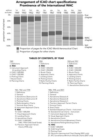
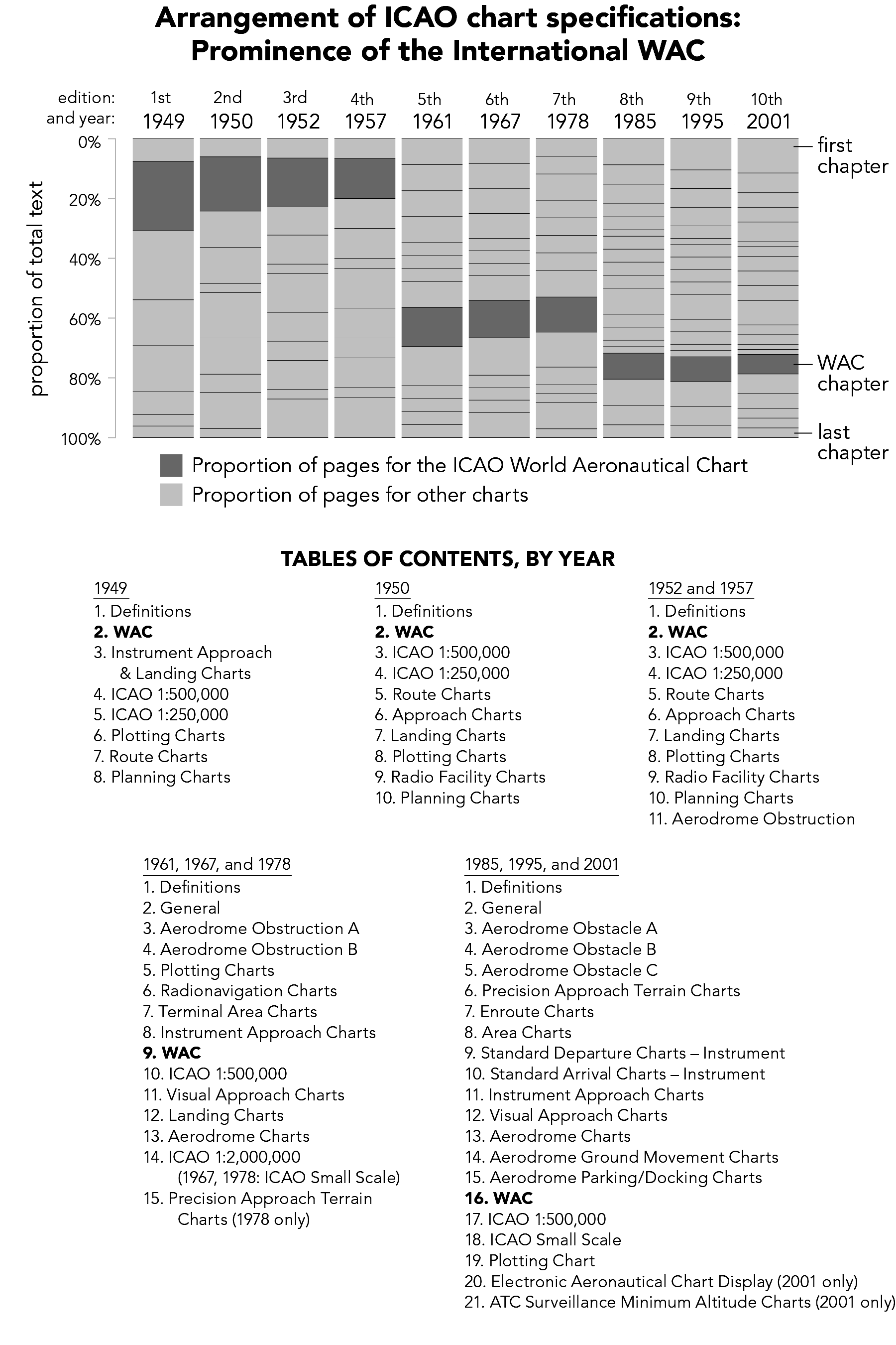
	FIGURE 2.19
	The place of the International World Aeronautical Chart in the official specifications of the International Civil Aviation Organization, 1949−2001
	William Rankin Creative Commons BY-NC-SA
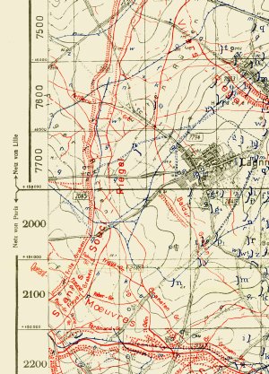
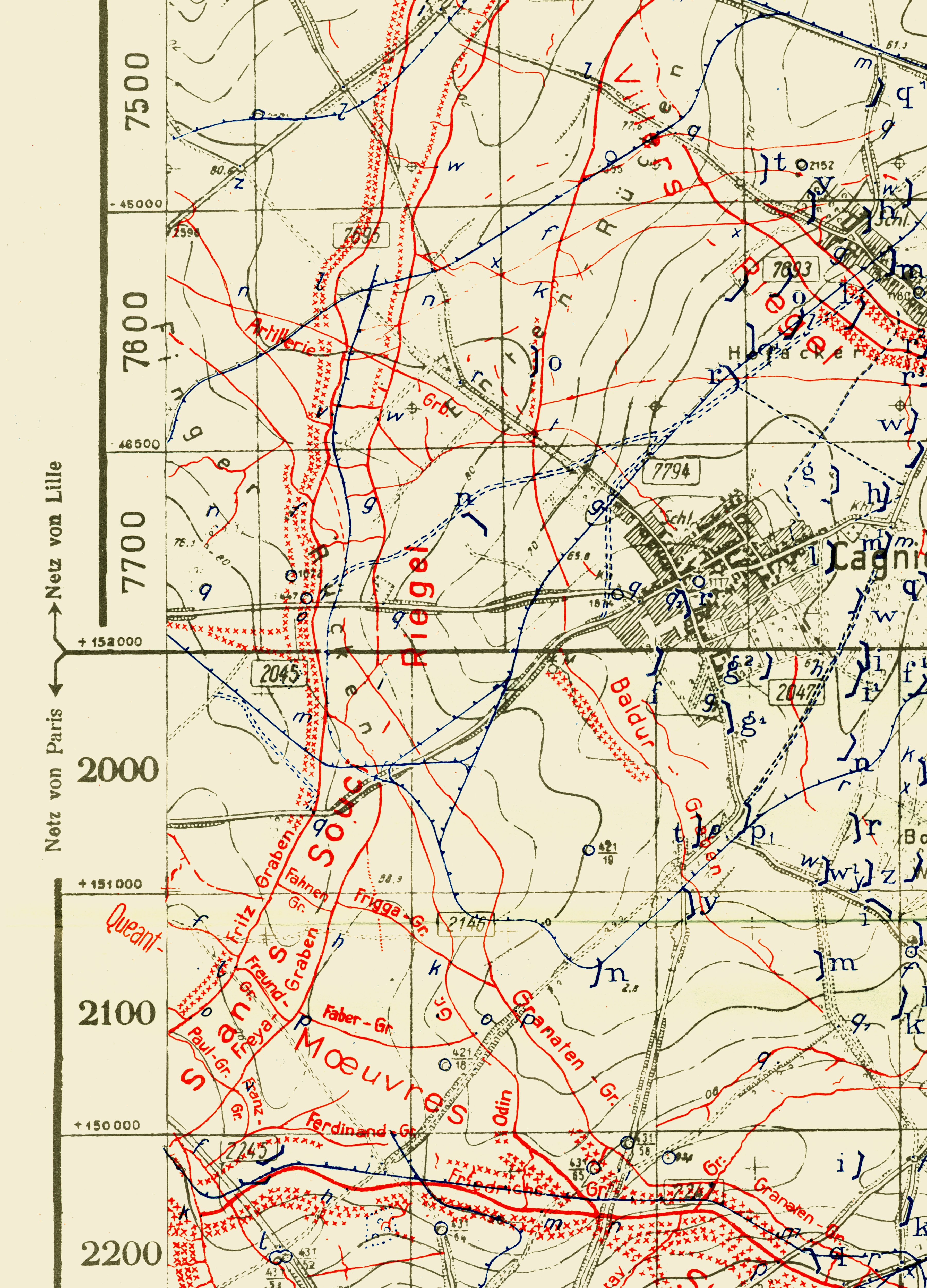
	FIGURE 3.1
	One-kilometer artillery grid on a French trench map, Moreuil, 5 Aug 1918
	Service Géographique de l’Armée Public Domain: copyright expired
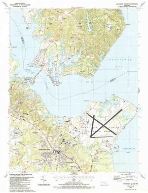
	FIGURE 3.2
	Universal Transverse Mercator grid on a US topographic map, Solomons Island, 1987
	US Geological Survey Public Domain: US government
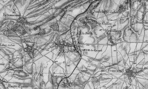
	FIGURE 3.3
	Detail from the French carte de l’État major, 1885
	Dépôt de la Guerre Public Domain: copyright expired
	FIGURE 3.4
	The Bonne projection used for the carte de l’État major, extended to show the entire world
	William Rankin Creative Commons BY-NC-SA
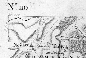
	FIGURE 3.5
	Sheet corner from Cassini's Carte de France, Verdun, 1760
	César-François Cassini de Thury Public Domain: copyright expired
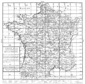
	FIGURE 3.6
	Index sheet from Cassini's Carte de France, 1797
	César-François Cassini de Thury Public Domain: copyright expired
	FIGURE 3.7
	Grid junctions on a German trench Map, Bourlon, 18 Sep 1918
	reproduced in Oskar Albrecht, Das Kriegsvermessungswesen während des Weltkrieges 1914–18 (München: Bayerische Akademie der Wissenschaften, 1969) Public Domain: copyright expired
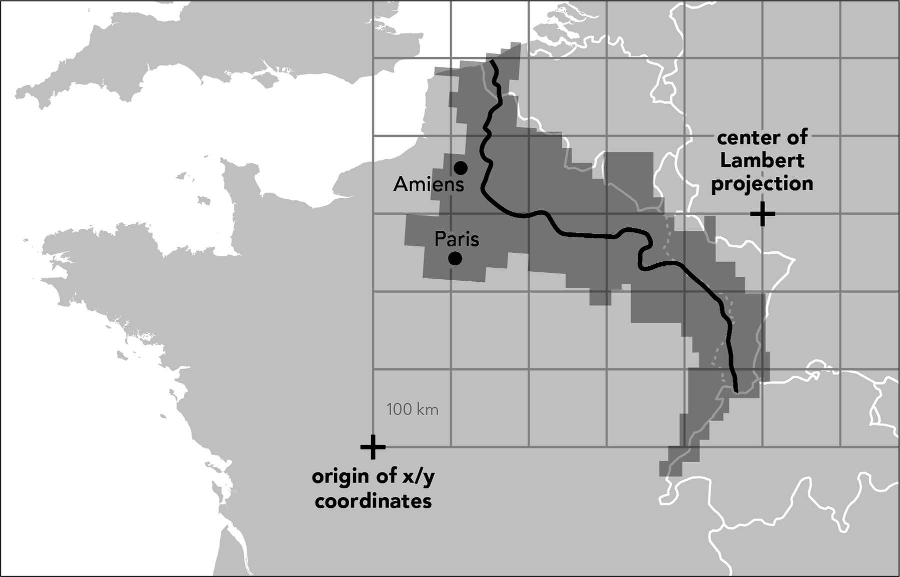
	FIGURE 3.8
	Deployment of the French système Lambert map grid along the western front
	William Rankin Creative Commons BY-NC-SA
	FIGURE 3.9
	The Lambert projection used for the système Lambert, extended to show the entire world
	William Rankin Creative Commons BY-NC-SA
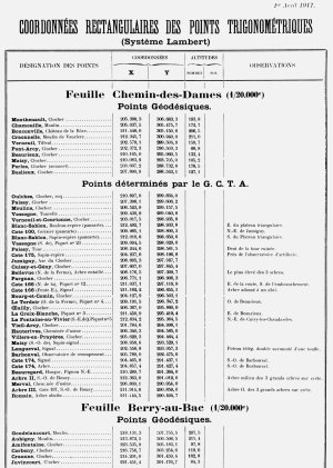
	FIGURE 3.10
	Page from a French trig list, April 1917, giving grid coordinates
	Service Géographique de l’Armée; reproduced in Peter Chasseaud, Artillery’s Astrologers: A History of British Survey & Mapping on the Western Front, 1914–1918 (Lewes: Mapbooks, 1999), 514 Public Domain: copyright expired
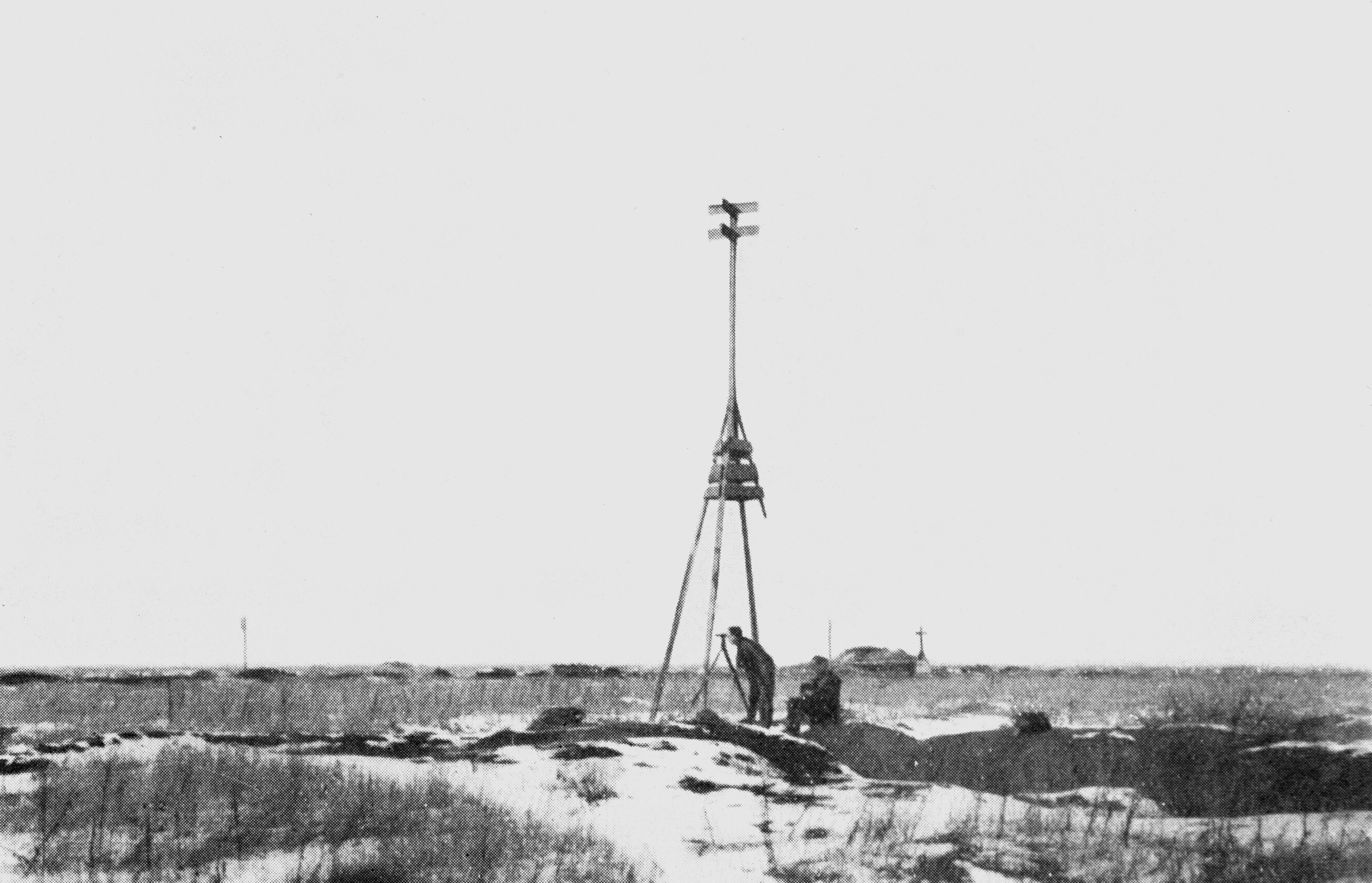
	FIGURE 3.11
	British surveyors measuring a captured German trig beacon during World War I
	from H. Winterbotham, “Geographical Work with the Army in France,” The Geographical Journal 54 (July 1919), 13 Public Domain: copyright expired
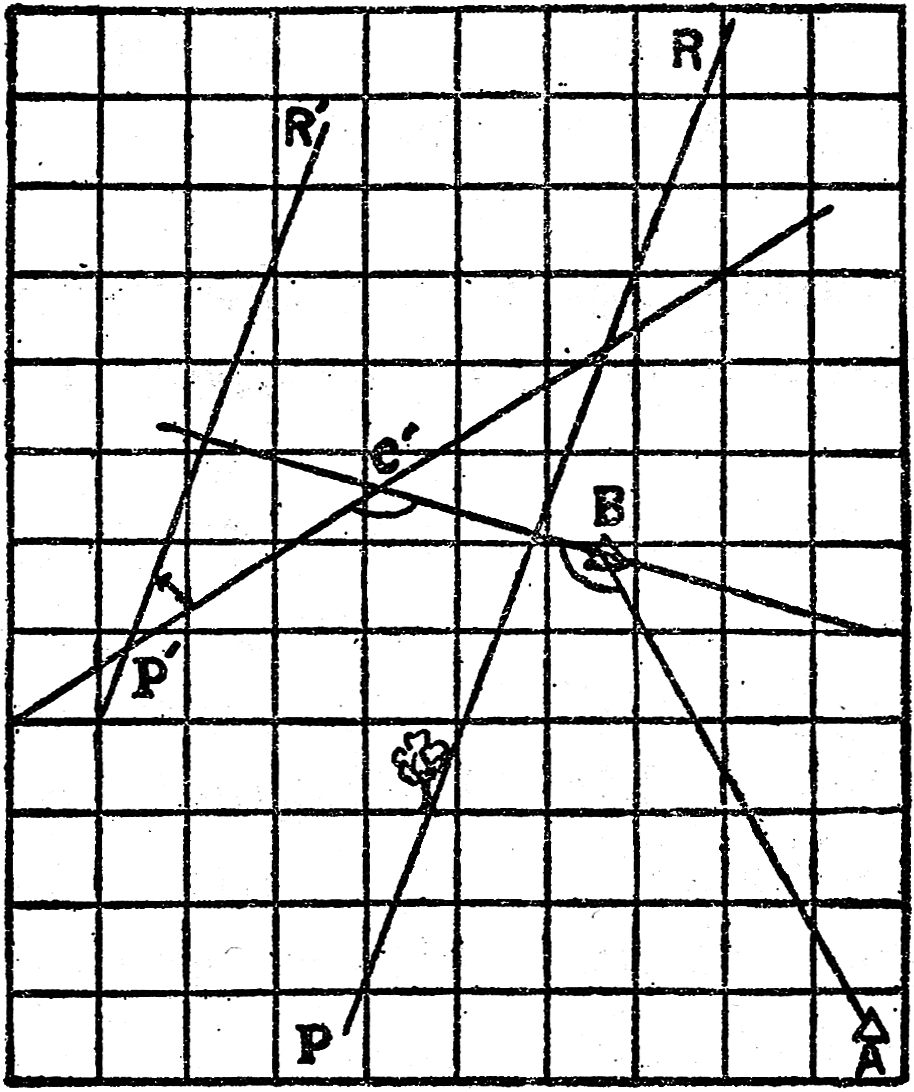
	FIGURE 3.12
	Textbook demonstration of how to plot a target on a plotting board
	from Manual for the Artillery Orientation Officer [translated from French original] (Washington DC: USGPO, 1917), 100 Public Domain: copyright expired
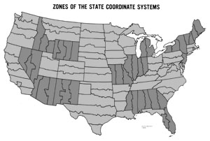
	FIGURE 3.13
	Zones of the US State Plane Coordinate System, with a separate grid system for each zone
	Surveying and Mapping Copyright 1967
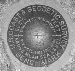
	FIGURE 3.14
	Survey monument in Mt. Vernon, Texas, placed in 1934
	QuesterMark Creative Commons BY-SA
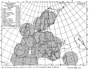
	FIGURE 3.15
	Henri Roussilhe’s scheme for an international grid system, 1922
	from H. Roussilhe, “Emploi des coordonnées rectangulaires stéréographiques pour le calcul de la triangulation dans un rayon de 560 kilomètres autour de l’origine,” Travaux de l’Association internationale de géodésie 1 (Paris, 1923 [presented 1922]); shading added Public Domain: copyright expired
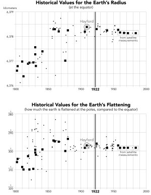
	FIGURE 3.16
	Historical values for the size and shape of the earth download data in a spreadsheet
	William Rankin Creative Commons BY-NC-SA
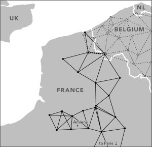
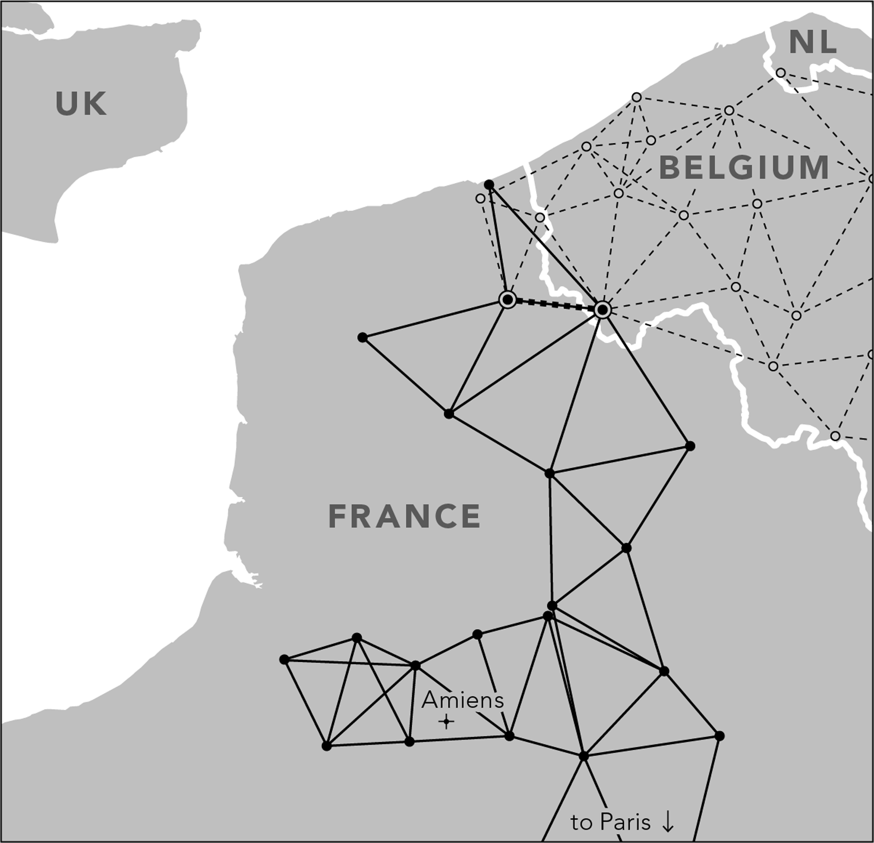
	FIGURE 3.17
	The junction of the French and Belgian national triangulations as of 1920
	William Rankin Creative Commons BY-NC-SA
	FIGURE 3.18
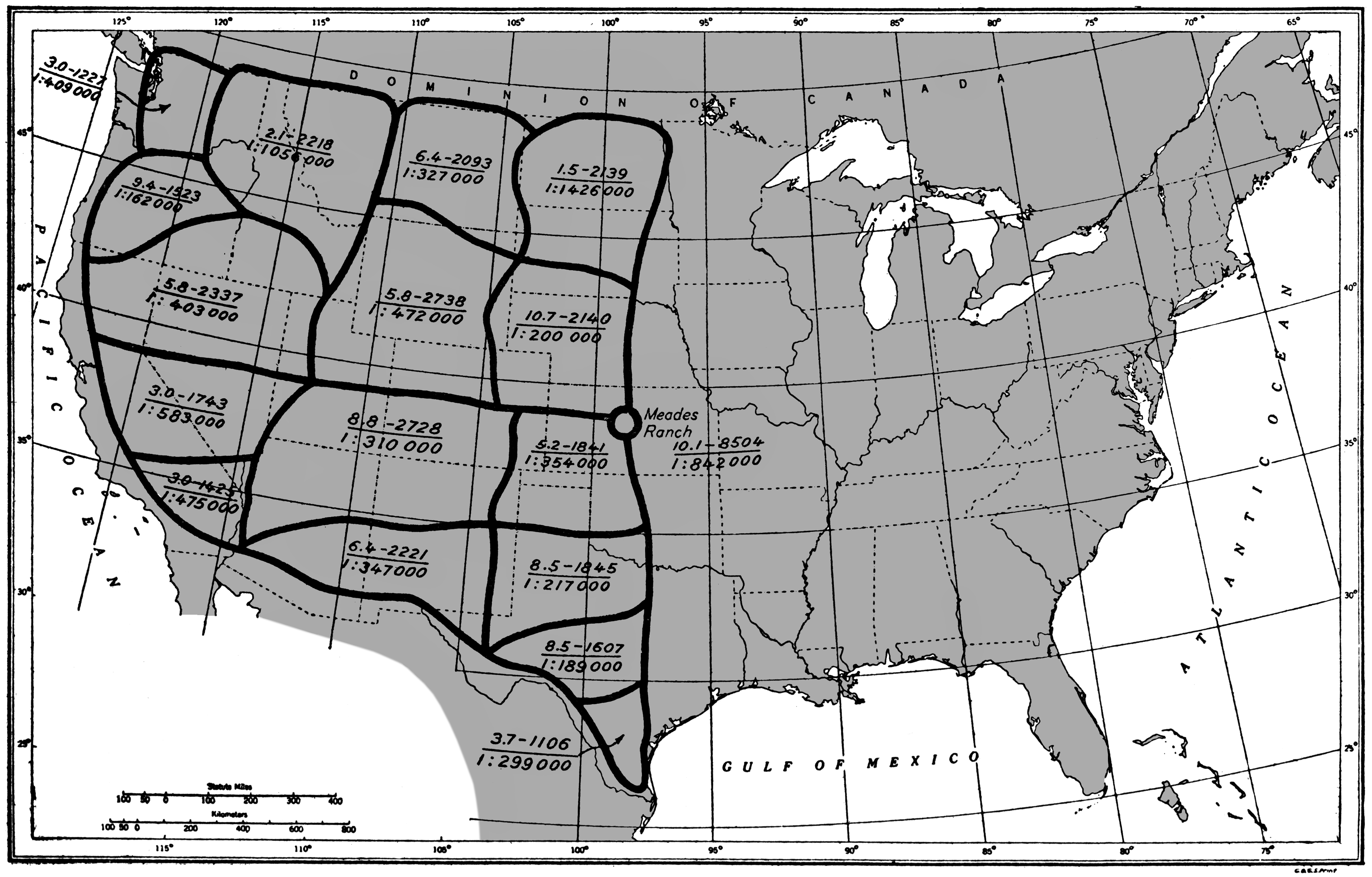
	The use of computationally efficient “Bowie Loops” in the western United States
	from Oscar Adams, The Bowie Method of Triangulation Adjustment, US Coast and Geodetic Survey special publication 159 (Washington, DC: USGPO, 1930), 10; shading added Public Domain: US government
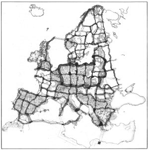
	FIGURE 3.19
	Schematic plan for the recalculation of the European triangulation network, 1939
	Bulletin géodésique Copyright 1939
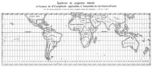
	FIGURE 3.20
	Pierre Tardi's plan for a grid system for Africa, 1936
	Bulletin géodésique Copyright 1938
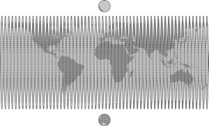
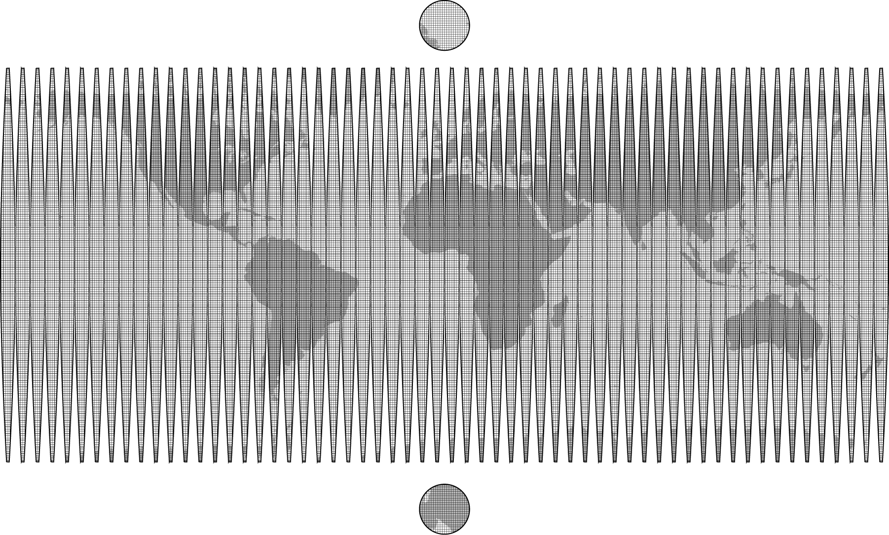
	FIGURE 4.1
	The Universal Transverse Mercator grid system, shown as if all maps were laid together like an unfolded globe download grid as a GIS layer
	William Rankin Creative Commons BY-NC-SA
	FIGURE 4.2
	Use of the Universal Transverse Mercator grid (and its Soviet counterpart) by the end of the Cold War
	William Rankin Creative Commons BY-NC-SA
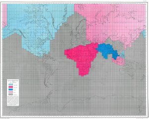
	FIGURES 4.3 AND 4.4
	British and American grids during World War II
	from US Army Map Service Memorandum No. 425, Grids and Magnetic Declinations, 2nd ed. (Washington DC, 1943); shading added Public Domain: US government
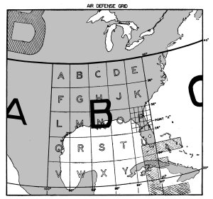
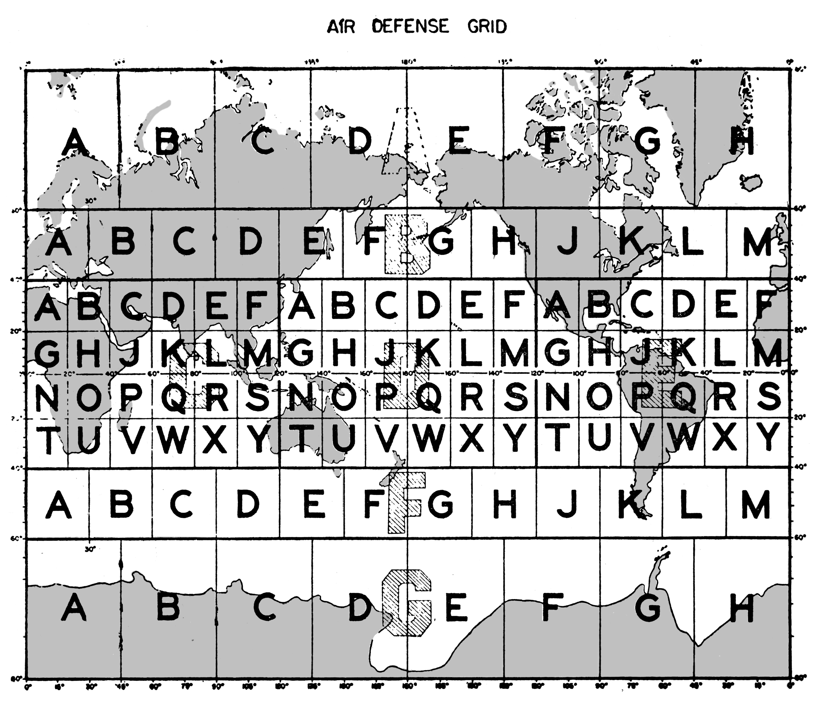
	FIGURE 4.5
	The first two reference levels of the US Air Defense Grid
	from War Department Technical Manual TM 44-225, Orientation for Artillery (Washington DC, 1944); shading added Public Domain: US government
	FIGURE 4.6
	The most precise references on the US Air Defense Grid
	from War Department Technical Manual TM 44-225, Orientation for Artillery (Washington DC, 1944); shading added Public Domain: US government
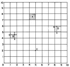
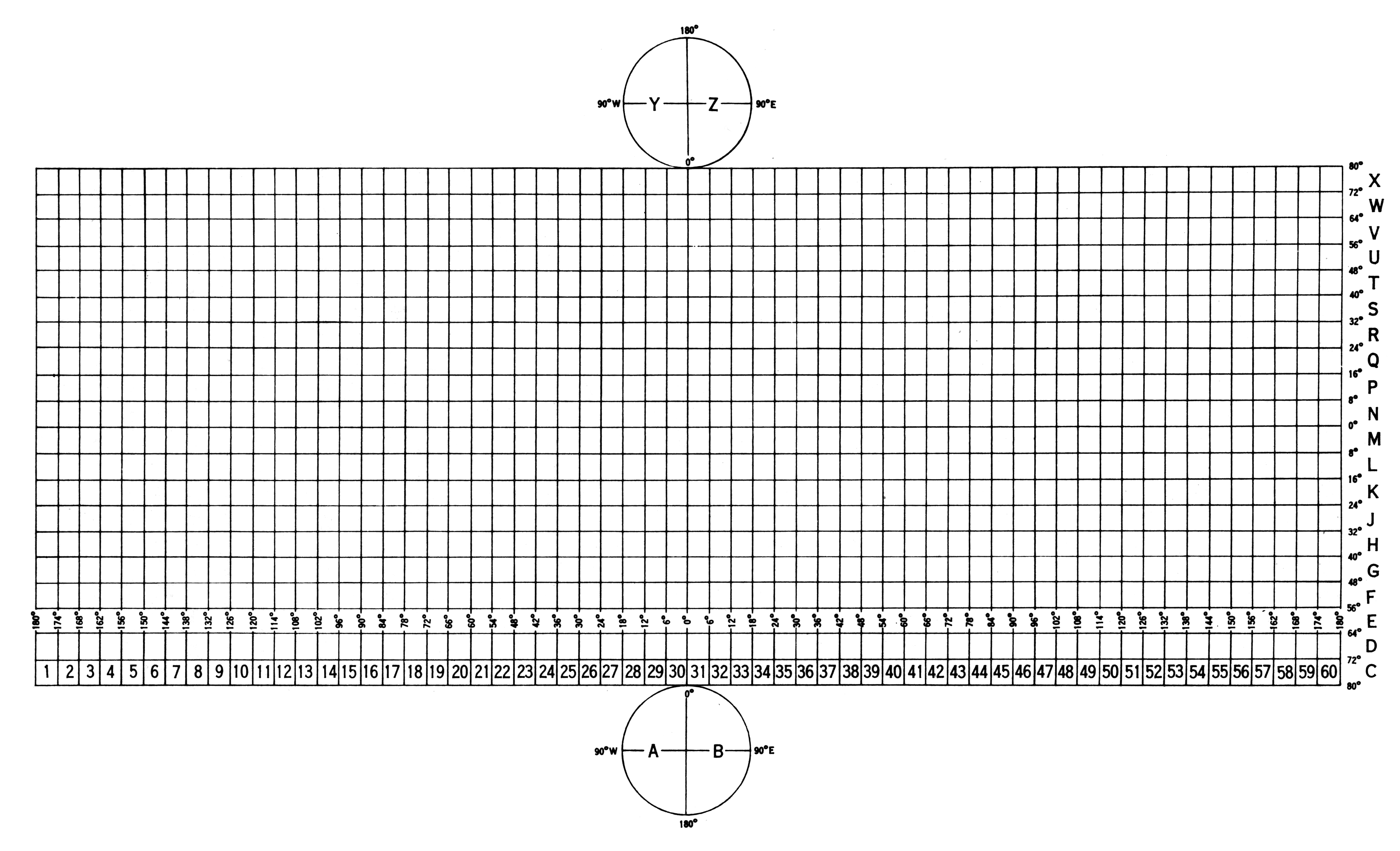
	FIGURE 4.7
	The US Joint Army–Navy reference system, applied to individual map sheets
	from War Department Technical Manual TM 44-225, Orientation for Artillery (Washington DC, 1944); shading added Public Domain: US government
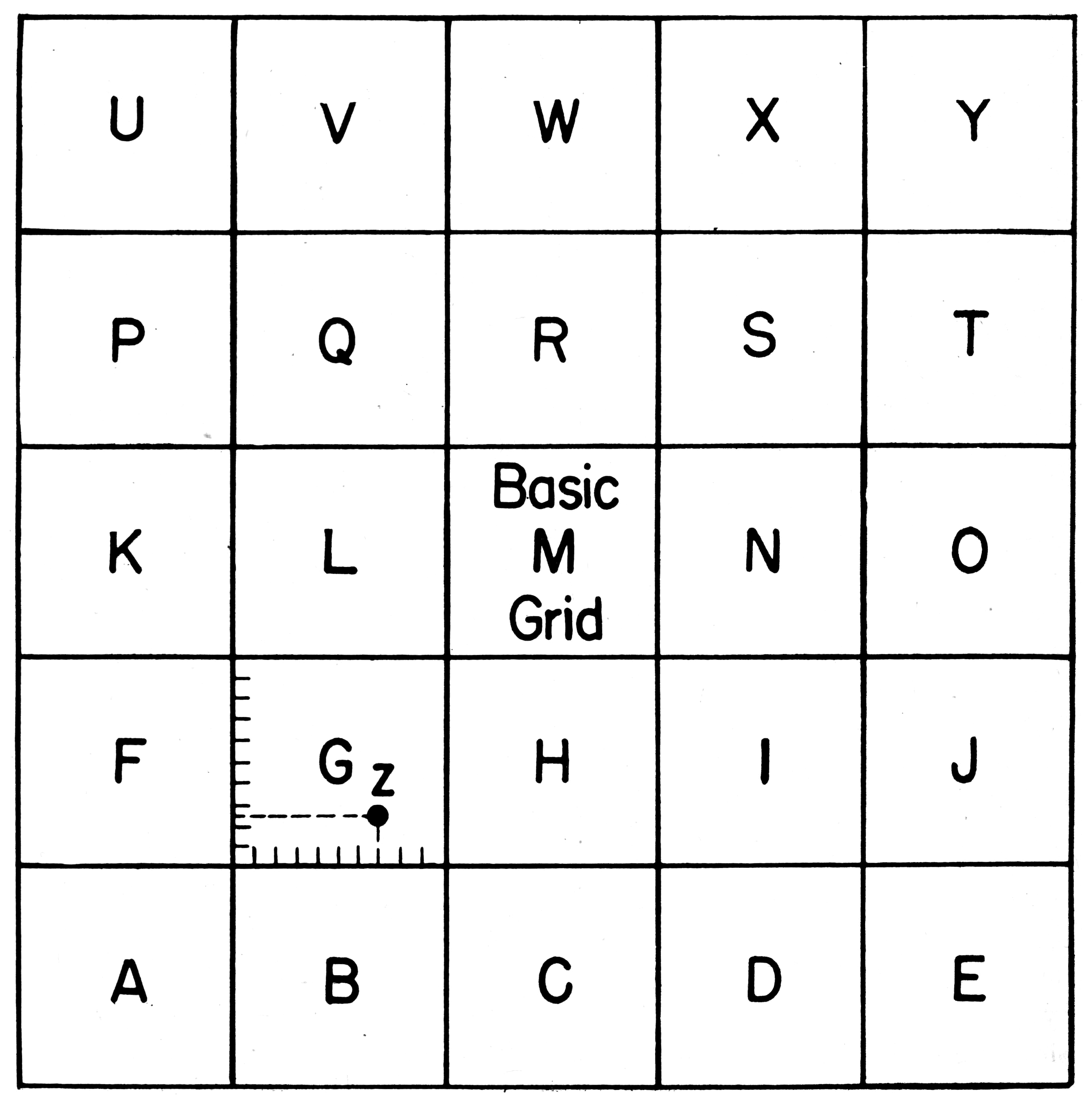
	FIGURE 4.8
	Expansion of the US Joint Army–Navy system to adjacent sheets (original map is square M)
	from War Department Technical Manual TM 44-225, Orientation for Artillery (Washington DC, 1944); shading added Public Domain: US government
	FIGURE 4.9
	Top-level “Grid Zone Designations” for the Universal Transverse Mercator grid
	from US Army Map Service Technical Manual No. 36, Grids and Grid References (Washington DC, 1950) Public Domain: US government
	FIGURE 4.10
	Grid Zones subdivided into 100-kilometer squares
	from US Army Map Service Technical Manual No. 36, Grids and Grid References (Washington DC, 1950) Public Domain: US government
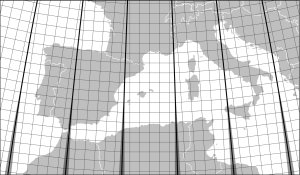
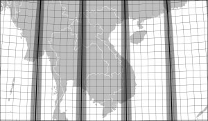
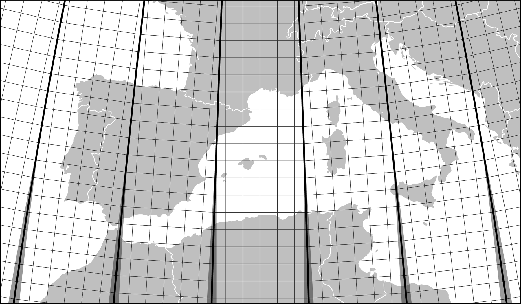
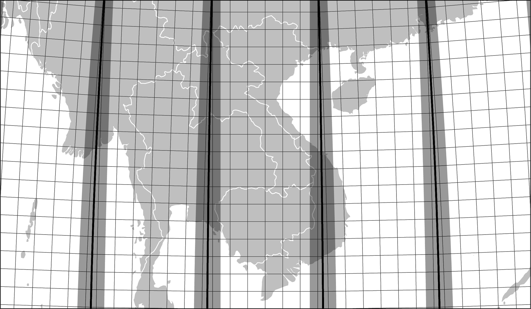
	FIGURE 4.11
	Areas of the Universal Transverse Mercator grid with high errors (in dark gray) for Europe and Southeast Asia download grid as a GIS layer
	William Rankin Creative Commons BY-NC-SA
	FIGURE 4.12
	Ellipsoids used for the Universal Transverse Mercator grid
	from US Army Map Service Technical Manual No. 7, Universal Transverse Mercator Grid Tables (Washington DC, 1949?) Public Domain: US government
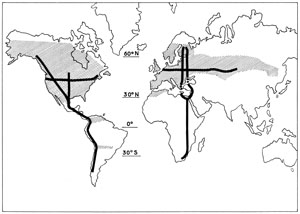
	FIGURE 4.13
	The US Army Map Service's scheme for recalculating the European triangulation, 1947
	from Floyd Hough, “The Readjustment of European Triangulation,” Transactions, American Geophysical Union 28 (Feb 1947), 63 Public Domain: copyright not renewed
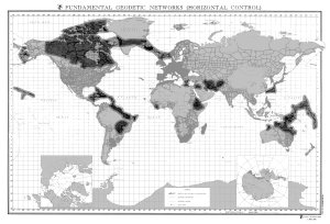
	FIGURE 4.14
	High-precision survey data used by the US Army Map Service to recalculate the size and shape of the earth in 1956
	Bulletin géodésique Copyright 1959
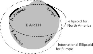
	FIGURE 4.15
	Mismatches between North-American and European values for the size and shape of the earth
	William Rankin, after Irene Fischer Creative Commons BY-NC-SA
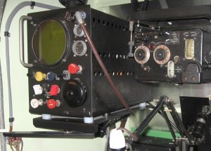
	FIGURE 5.1
	Mockup of a Gee receiver in an Avro Lancaster bomber
	photo by Peter Zijlstra used with permission
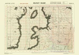
	FIGURE 5.2
	Gee lattice chart showing northern England, Wales, and eastern Ireland (postwar reprint of 1944 edition)
	British War Office Public Domain: expired Crown Copyright
	FIGURE 5.3
	A call for public investment in aviation: Buffalo, NY, 1927
	Buffalo Journal of Commerce Public Domain: copyright not renewed
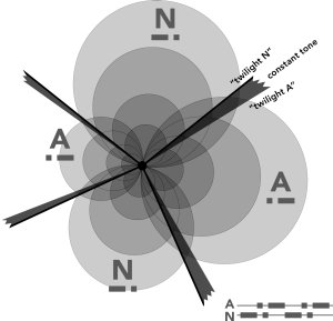
	FIGURE 5.4
	The directional Morse-code broadcasts of the US Radio Range create four narrow beams
	William Rankin Creative Commons BY-NC-SA
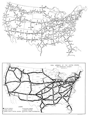
	FIGURE 5.5
	The network of Radio-Range airways in the United States in the late 1930s
	from Ronald Keen, Wireless Direction Finding, 3rd ed. (London: Iliffe & Sons, 1938), 484, and Civil Aeronautics Authority, First Annual Report of the Civil Aeronautics Authority (Washington: USGPO, 1940), appendix B Public Domain: US government
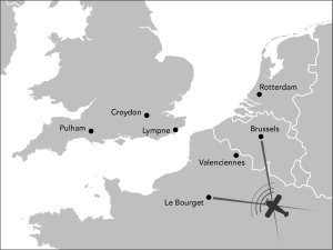
	FIGURE 5.6
	Radio Direction Finding (D/F) stations in Europe as of 1931
	William Rankin Creative Commons BY-NC-SA
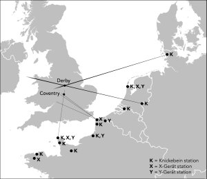
	FIGURE 5.7
	German beams aimed at the UK during the Battle of Britain, summer 1941
	William Rankin Creative Commons BY-NC-SA
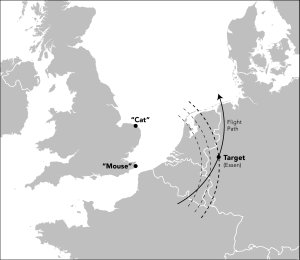
	FIGURE 5.8
	The British Oboe system, as configured for a bombing raid on Essen in 1942
	William Rankin Creative Commons BY-NC-SA
	FIGURE 5.9
	European coverage of the British Gee system at the end of World War II
	William Rankin Creative Commons BY-NC-SA
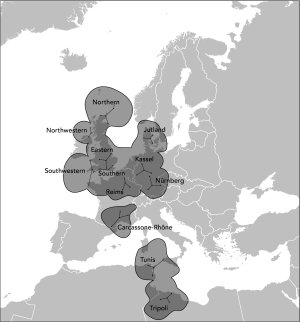
	FIGURE 5.10
	Coverage of the German Sonne system at the end of World War II
	William Rankin Creative Commons BY-NC-SA
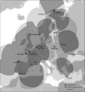
	FIGURE 5.11
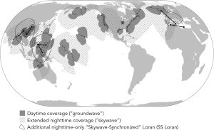
	Coverage of the American Loran system at the end of World War II download transmitter locations and chain connections as GIS layers
	William Rankin Creative Commons BY-NC-SA
	FIGURE 5.12
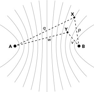
	Hyperbolic navigation: position is determined by measuring the time difference between signals sent from two synchronized transmitters
	William Rankin Creative Commons BY-NC-SA
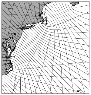
	FIGURE 5.13
	The hyperbolic grid of Loran off the east coast of the United States and Canada
	from J. A. Pierce, “An Introduction to Loran,” Proceedings of the IRE 34 (May 1946), 219; shading added Public Domain: copyright not renewed
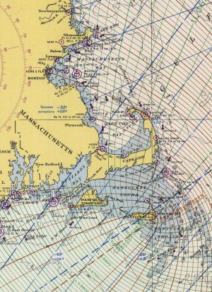
	FIGURE 5.14
	Detail of Loran Chart, Atlantic Coast: Cape Sable to Cape Hatteras, chart 1000-L (1948)
	US Coast and Geodetic Survey Public Domain: US government
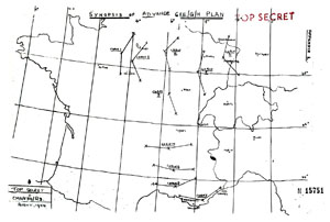
	FIGURE 5.15
	Plan for advancing Gee coverage in France and Germany after D-Day
	British War Office Copyright 1944
	FIGURE 5.16
	Trilateration surveying with Shoran after World War II
	from Carl Aslakson, “The Influence of Electronics on Surveying and Mapping,” Surveying and Mapping (July–Sept 1950), 167 Public Domain: copyright not renewed
	FIGURE 5.17
	Trilateration performed during the 1950s and 1960s (shaded in gray)
	from Defense Mapping Agency, Geodesy for the Layman, 5th ed. (Washington: DMA, 1983; map dated 1971), 18; shading added Public Domain: US government
	FIGURE 5.18
	Advertisement for offshore radio surveying, 1959
	from Surveying and Mapping (Mar 1959), 141 Public Domain: copyright not renewed
	FIGURE 5.19
	Advertisement for offshore radio surveying, 1971
	Surveying and Mapping Copyright 1971
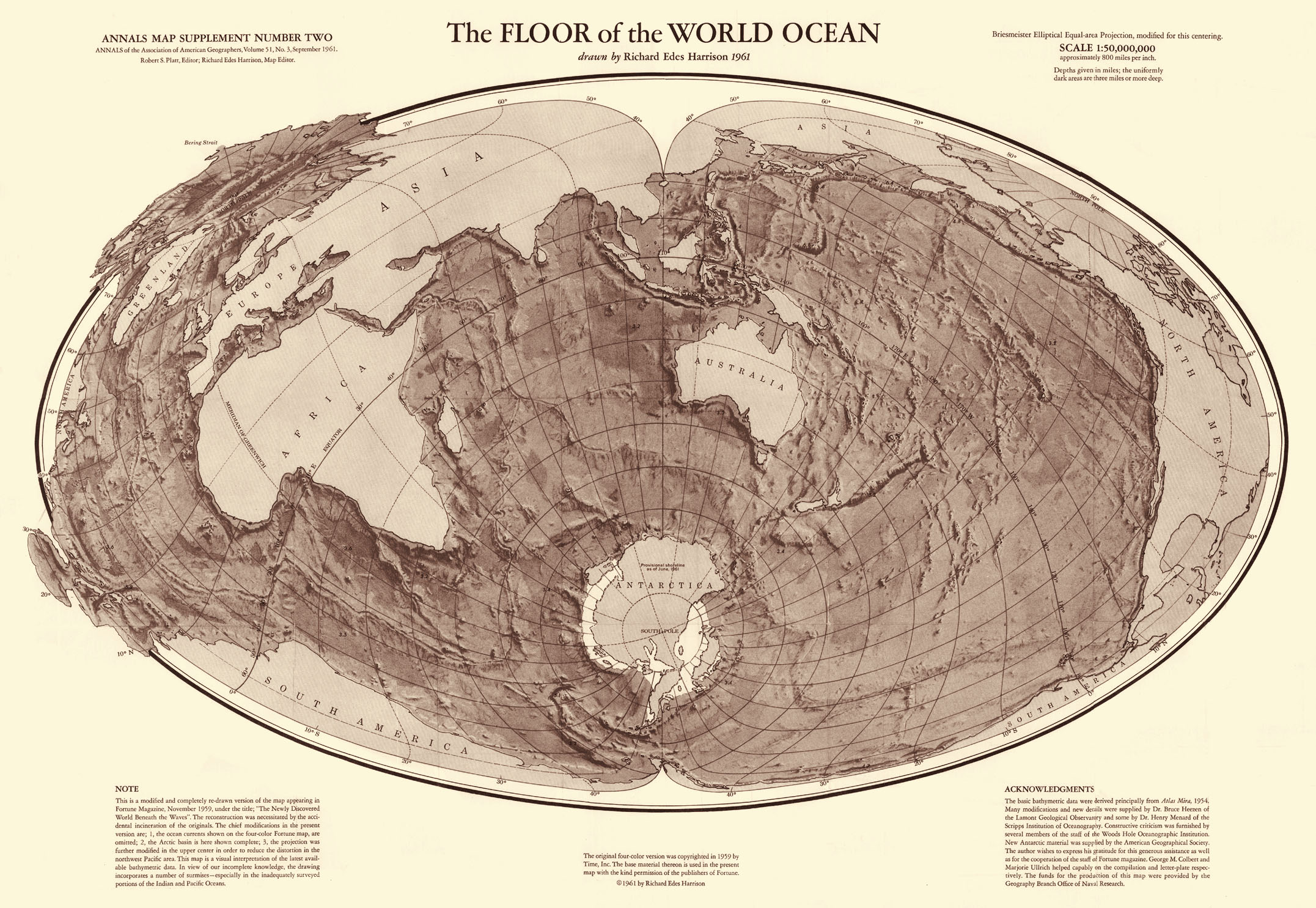
	FIGURE 5.20
	The Floor of the World Ocean, by Richard Edes Harrison (1961 version of 1959 original)
	from Annals of the Association of American Geographers 51 (Sept 1961) Public Domain: copyright not renewed
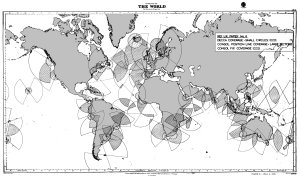
	FIGURE 5.21
	British proposal for worldwide Consol and Decca coverage, 1947
	from International Meeting on Marine Radio Aids to Navigation: Proceedings and Related Documents, April 28 – May 9, 1947 (Washington: State Department, 1948), facing 438; shading added Public Domain: US government
	FIGURE 5.22
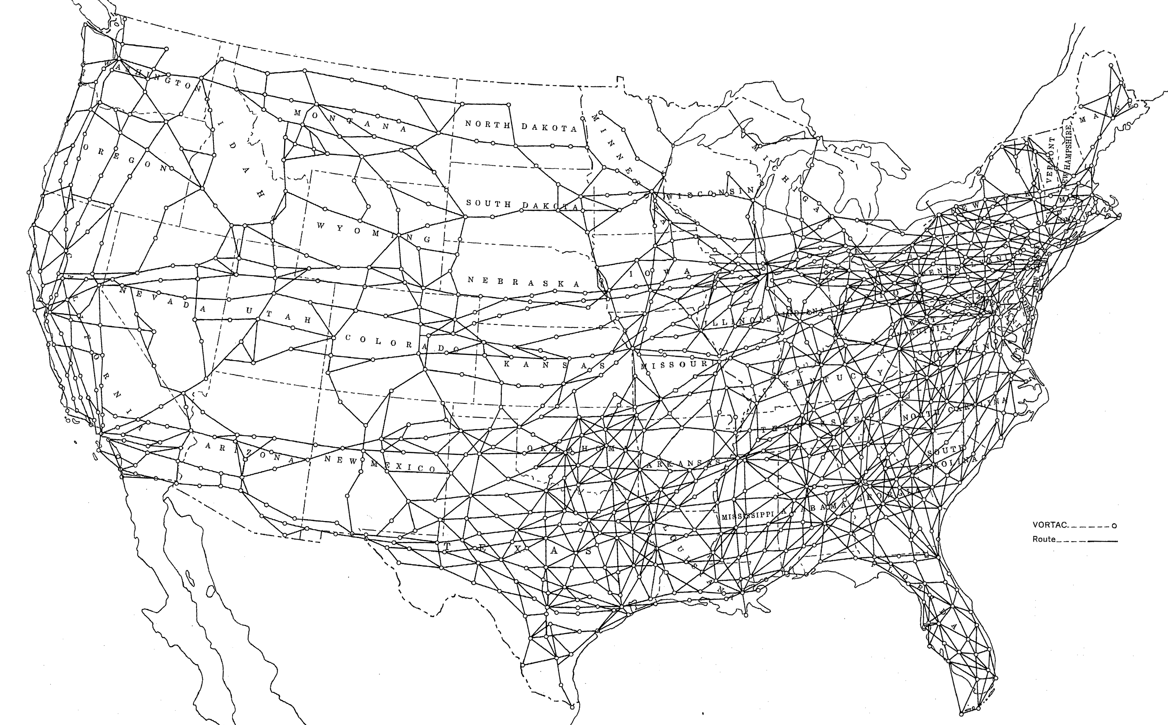
	1959 US plan for the VOR/DME airway network through 1965
	from US Air Coordinating Committee Technical Division, “Short Distance Radionavigation: Background Information and Views Presented by the United States of America,” 1958 (ICAO, box “SP/COM/OPS/RAC 1958”), chart 9 Public Domain: US government
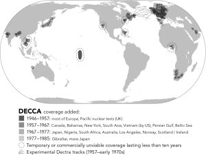
	FIGURE 5.23
	Expansion of Decca coverage, 1946–1985 download transmitter locations and chain connections as GIS layers
	William Rankin Creative Commons BY-NC-SA
	FIGURE 5.24
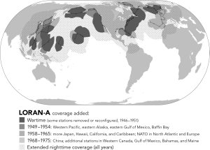
	Expansion of Loran-A coverage, 1946–1975 download transmitter locations and chain connections as GIS layers
	William Rankin Creative Commons BY-NC-SA
	FIGURE 5.25
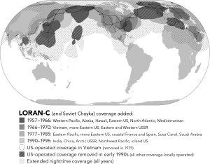
	Expansion (and contraction) of Loran-C coverage, 1957–1996 download transmitter locations and chain connections as GIS layers
	William Rankin Creative Commons BY-NC-SA
	FIGURE 5.26
	Integrated map display with a fixed map and a movable "bug" showing the pilot's real-time location (1965)
	Navigation (US) Copyright 1965
	FIGURE 5.27
	A palm-sized "roller map" display that would automatically advance as the plane followed its course (1960)
	Journal of the Institute of Navigation (UK) Copyright 1960
	FIGURE 6.1
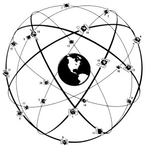
	GPS satellite constellation design, mid-1980s
	from R. L. Beard, J. Murray, and J. D. White, “GPS Clock Technology and the Navy PTTI Programs at the U.S. Naval Research Laboratory,” in Proceedings of the Eighteenth Annual Precise Time and Time Interval (PTTI) Applications and Planning Meeting (1986), 50 Public Domain: US government
	FIGURE 6.2
	A GPS collar on “Floggy,” a brown hyena, in Namibia in 2006
	photo by Ingrid Wiesel, from “Predicting the influence of land development on brown hyena (Parahyaena brunnea) movement and activity” used with permission
	FIGURE 6.3
	The "birdcage" of the US Navy's Transit satellites
	Navigation (US) Copyright 1978
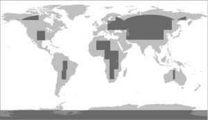
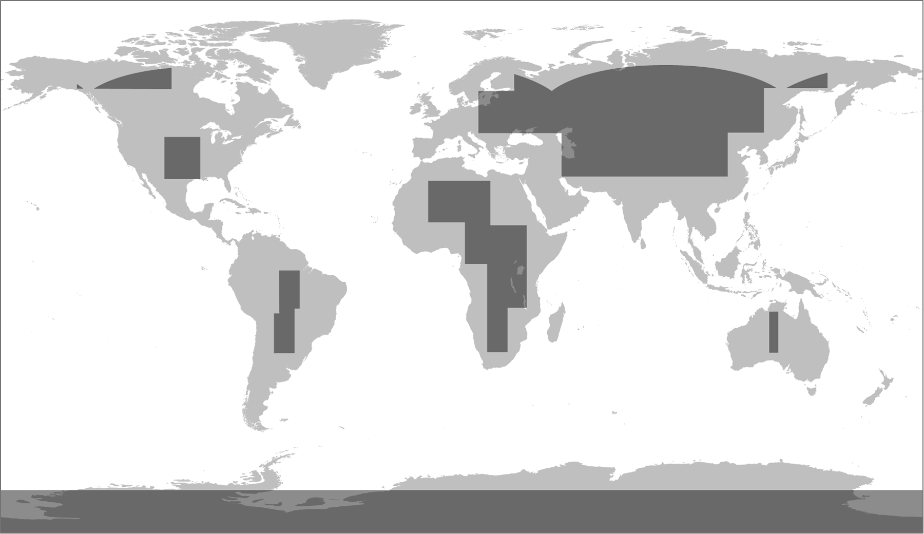
	FIGURE 6.4
	Coverage of Omega lattice charts in the early 1970s: maps were not available gray areas
	William Rankin Creative Commons BY-NC-SA
	FIGURE 6.5
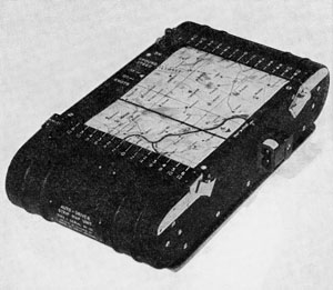
	The US Navy's AN/UYK-1 computer for Transit satellite navigation, circa 1961
	from Ramo-Woolridge (a division of TRW), AN/UYK-1: A Multiple Purpose Digital Computer, 21 Apr 1961 Public Domain: no copyright notice
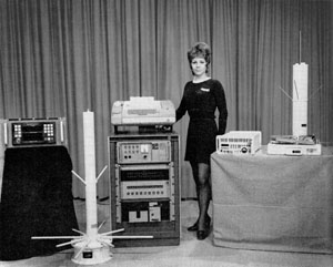
	FIGURE 6.6
	Shrinking Transit equipment from Magnavox, 1968 to 1976
	Navigation (US) Copyright 1971, 1978
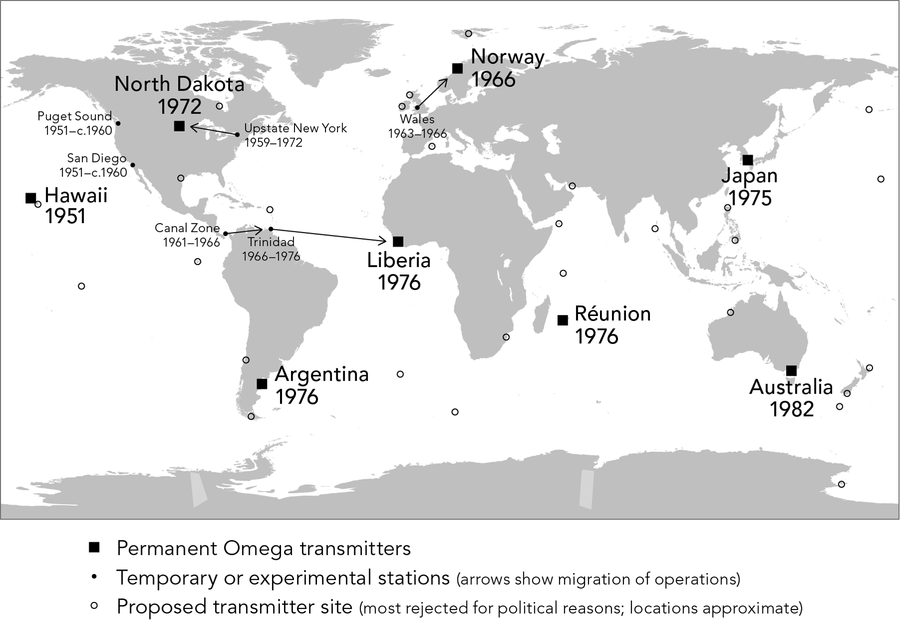
	FIGURE 6.7
	Omega transmitter locations, 1951–1997 download locations as a GIS layer
	William Rankin Creative Commons BY-NC-SA
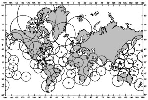
	FIGURE 6.8
	Proposed network of Omega monitoring stations as of 1978
	Navigation (US) Copyright 1978
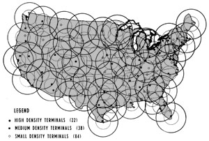
	FIGURE 6.9
	A 1975 proposal for “differential” Omega stations in the contiguous United States
	Navigation (US) Copyright 1975
	FIGURE 6.10
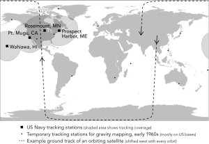
	Ground installations for the Transit satellite system
	William Rankin Creative Commons BY-NC-SA
	FIGURE 6.11
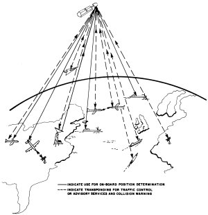
	A civilian satellite-navigation system designed for NASA, circa 1970
	from Leo M. Keane et al., “Global Navigation and Traffic Control Using Satellites,” NASA Technical Report R-342, July 1970,12 Public Domain: US government
	FIGURE 6.12
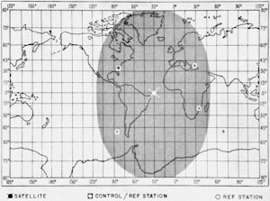
	A plan for megaregional coverage for a civilian satellite navigation system in a geostationary orbit, mid-1960s
	Navigation (US) Copyright 1966
	FIGURE 6.13
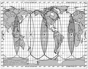
	A plan for near-global civilian coverage from six geostationary satellites, mid-1960s
	Navigation (US) Copyright 1967
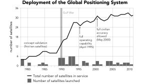
	FIGURE 6.14
	Launch and operational status of GPS satellites, 1978–2010 download data in a spreadsheet
	William Rankin Creative Commons BY-NC-SA
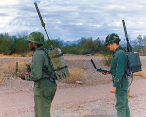
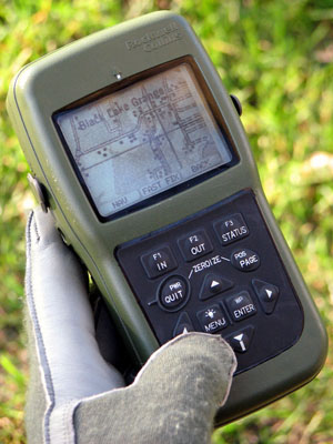
	FIGURE 6.15
	The shrinking size of GPS equipment: the "Manpack" of 1978 compared with the DAGR of 2004
	from Steven Lazar, “Modernization and the Move to GPS III,” Crosslink 3 (Summer 2002), 45, and Rockwell Collins, Inc. Copyright 1978?, 2008?
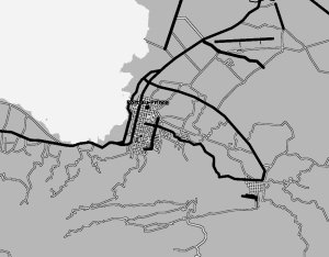
	FIGURE 6.16
	OpenStreetMap data, before and after the 2010 Haiti earthquake
	adapted from Mikel Maron's screencaptures Creative Commons BY-SA
	FIGURE 6.17
	Shindand airfield, Afghanistan, after an American GPS-guided bomb strike, October 2001
	US Department of Defense Public Domain: US government
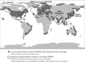
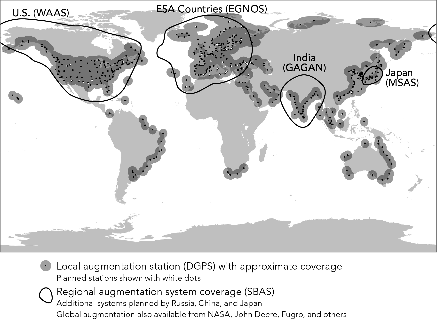
	FIGURE 6.18
	GPS augmentation systems as of 2015: Differential GPS (DGPS) and Satellite-Based Augmentation Systems (SBAS) download DGPS as GIS layers
	William Rankin Creative Commons BY-NC-SA
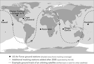
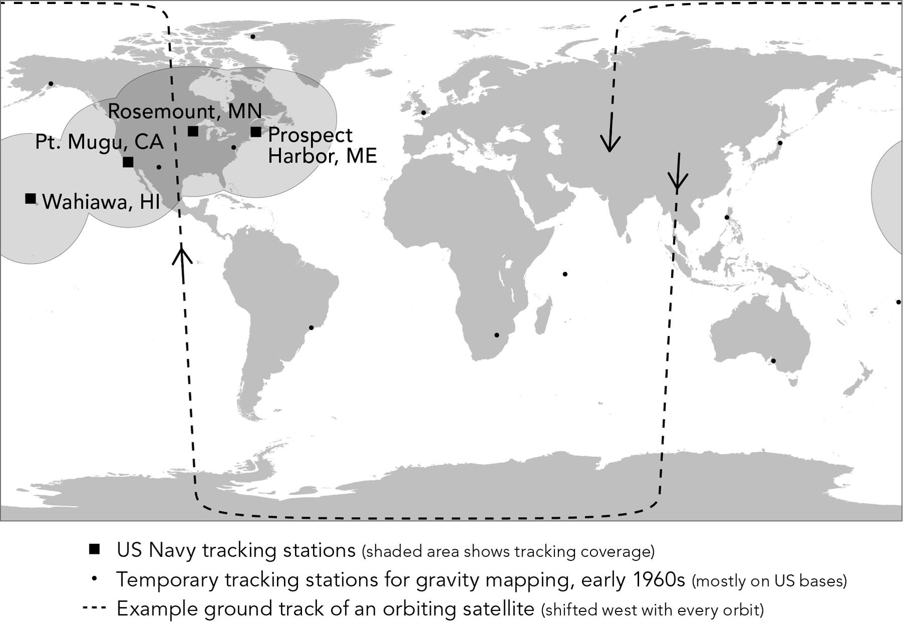
	FIGURE 6.19
	GPS ground installations: original US-controlled sites, with more recent stations in other countries
	William Rankin Creative Commons BY-NC-SA